NR Protocol Stack: PHY
The MAC layer is responsible for the construction of the transport block, and this includes both the data and control elements.
The job of the PHY layer is to transmit the transport block over the wireless channel as efficiently as possible. The PHY layer does this, with the help of functions like channel coding, modulation, multi-antenna processing and by mapping the physical time and frequency resources in the appropriate signals.
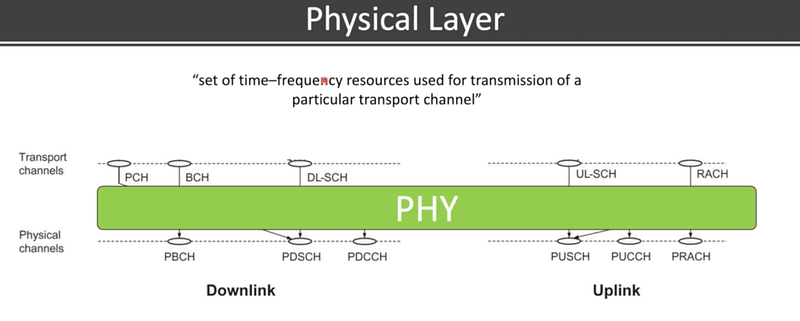
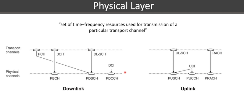
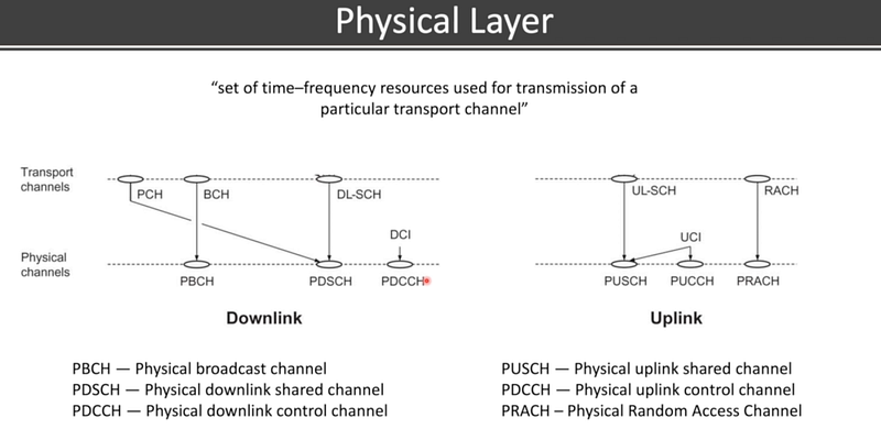
A physical channel corresponds to a set of time and frequency resources that is used for transmitting the transport block.
Each transport channel is mapped to a corresponding physical channel whereas there are some physical channels that do not correspond to any of the transport channels. These channels are called layer1 and layer2 control channels. This includes DCI (downlink control information) which provides the device with the necessary information for the proper functioning of decoding and demanding data. This also includes UCI which provides the scheduler on the hybrid scheduler
The PHY layer is the most sophisticated layer and it involves a lot a functions.
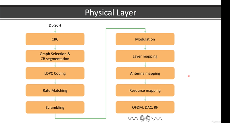
CRC
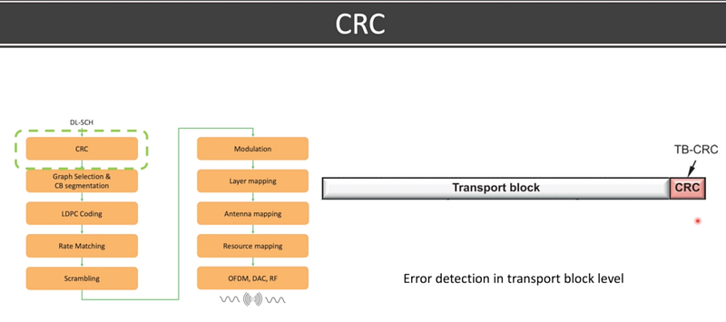
CRC (Cyclic Redundancy Check) is a mechanism to detect errors on the level of the transport block. For this purpose, CRC is calculated and added to the transport block. On the receiver side, the CRC can be used to detect any errors in the transport block level and request retransmissions if the transport block is not fully correct. The CRC length can vary according to the transport block size.
Graph selection and CB segmentation
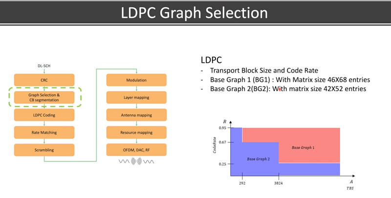
When it comes to channel coding which is used for error correction, NR uses LDPC (Low-density parity check) coding. LDPC is used for data channels and polar coding is used for control channels.
LDPC coding uses a parameter called a base graph that governs the coding process. NR supports the 2 LDPC-based graphs, 1 for the small transport block and 1 for the large transport block.
The LDPC base graph type is determined by 2 parameters, 1 is the size of the transport block and 2nd is the coding rate.
When the size of the transport block or the coding rate is above a certain threshold then base graph 1 is obtained. Otherwise, base graph 2 is used. Base graph 1 is used for large transport blocks or high coding rates. Similarly, base graph 2 is used for small transport blocks or low coding rates.
The transport block can be quite big, but the LDPC coding has a maximum code block size to limit the computational complexity. So if the transport block is bigger than this limit, it has to be segmented into smaller blocks called code blocks before the LDPC coding is performed.
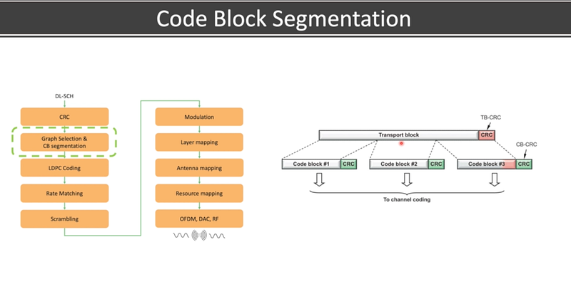
The transport block is segmented into the size of code blocks and CRC is added to each code block.
This segmentation is necessary before LDPC coding can be applied because the transport block size is too big to apply LDPC on it.
The CRC on the code block level might seem redundant compared to the CRC on the transport block-level but NR supports retransmitting just the erroneous code blocks instead of transmitting the whole transport block.
When the error occurs on a small level then instead of transmitting the whole transport block, only the code block containing the error would be retransmitted. we should be able to say exactly which code block the error was in. This will increase efficiency.
So we need an error detection method that is granular to the extent of code block level. So for this purpose, another CRC is added to each code block.
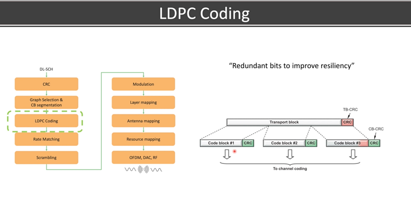
LDPC Coding
As CRC helps in error detection, similarly LDPC coding helps in error correction. Channel coding is the process of adding additional bits to improve resiliency. So in this step, we take each code block and apply LDPC coding to improve the resiliency and to be able to correct some of the smaller errors.
Rate Matching
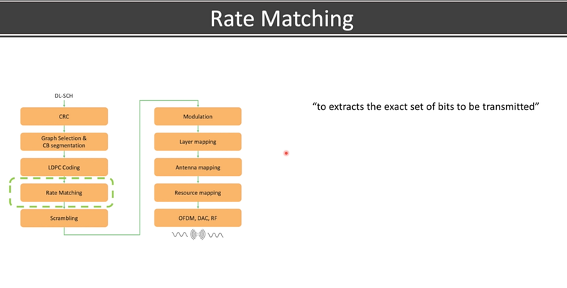
Not all of the output of the LDPC coding step can be transmitted in a given transmission time interval. So after the LDPC coding, rate matching takes the coded bits and extracts the exact set of bits that can be transmitted in a given transmission time interval.
Rate matching is performed with each code block.
Scrambling
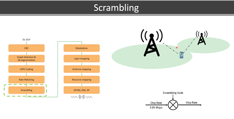
A UE may hear signals from multiple gNBs simultaneously. To be able to differentiate the incoming signals into separate gNBs at the very low layers of the protocol stack because in the high layers,we have different ways of addressing the device. But at the physical layer level, the device needs a mechanism so that it can receive signals from 1 gNB at a time and ignore the signals coming from the interfering gNBs.
So in scrambling, a block of code is multiplied by a scrambling sequence. Now the device that knows the scrambling sequence can see the information corresponding to the correct gNB as a signal but all the interfering gNBs use different scrambling sequences, so as a consequence the signals coming from the other gNBs will look like a pure noise to the UE.
So in this way, the UE listens to 1 gNB and treats all other gNBs as interference and noise.
So without DL scrambling, the channel coding at the device could find it difficult to differentiate the interfering signals. But by applying different scrambling sequences for neighboring cells, the interfering signals are randomized and the UE will be able to differentiate what is the desired signal and what is the interfering signal.
Modulation
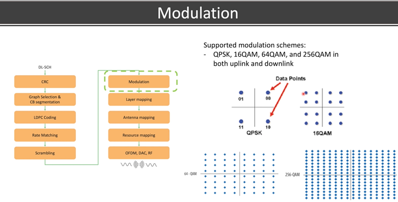
After scrambling is done, it’s the time for the actual IQ modulation.
In downlink data modulation, we transform the block of scrambled bits from ones and zeros to corresponding complex modulation symbols.
1 symbol represents n bits depending on the modulation type that’s used.
Layer Mapping
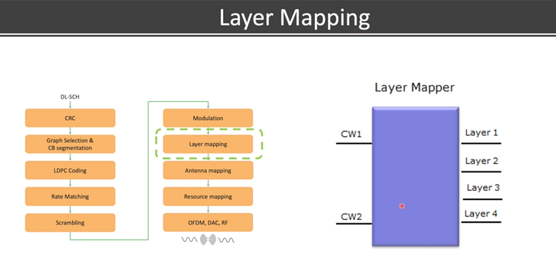
NR supports multiplexing, which means that it can transmit more than 1 layer of data simultaneously using the benefits of multiple antenna technologies. Since many of the NR radios include multiple antennas, it is often possible that multiple layers are supported.
So in-depth, the complex value modulation symbols that need to be transmitted are mapped into 1 or more layers.
The incoming symbols are mapped to the corresponding layers.
Antenna Mapping and Precoding
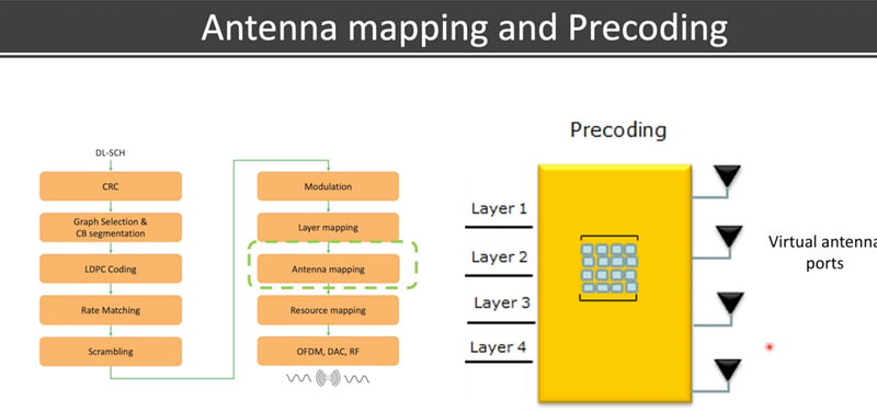
After mapping to different layers, the next step is to map the corresponding virtual antenna ports.
The precoding is based on the channel conditions; the precoding process maps the different number of layers into the corresponding no. of virtual ports. This uses a precoding matrix.
Precoding is the process that helps to use multiple antenna systems and understanding the channel knowledge to make multiple layers possible.
Resource and physical antenna mapping
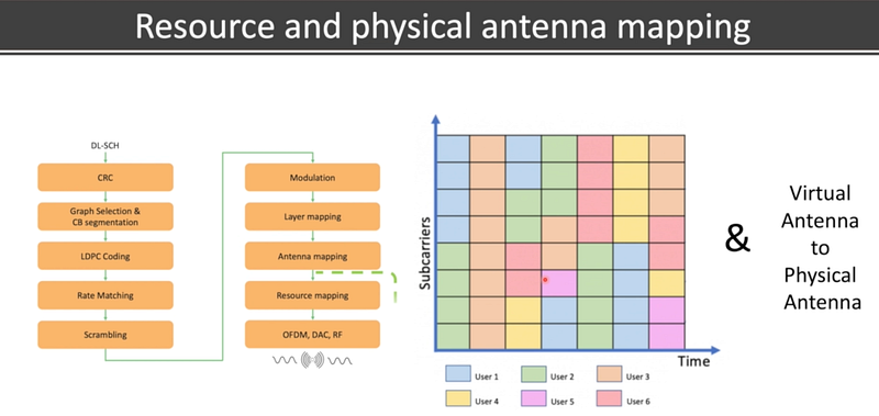
From the previous step of antenna mapping, we have the symbols for each virtual antenna port.
The resource block mapping takes the modulation symbols to be transmitted on each antenna port and maps to the set of resource elements in the set of resource blocks assigned by the MAC scheduler for current transmission.
The resource blocks are shared together with control signals and reference signals. The other resource blocks are used for the actual data transmission. So the no. of physical antennas is usually larger than the no. of virtual antenna ports which are used in the precoding stage.
So a linear mapping is applied to map from the virtual antenna port to the physical antenna ports. We take the data that is mapped to different virtual antenna ports and put them in the right time and frequency resource blocks which correspond to the decisions made by the scheduler.
OFDM, DAC, RF
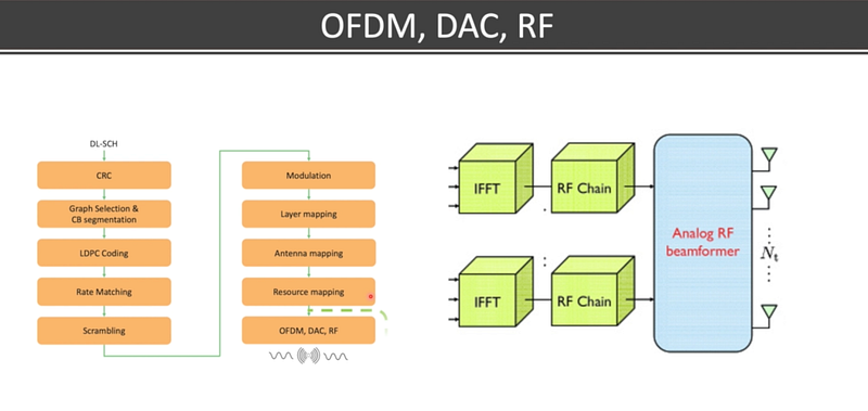
The symbols are mapped to the OFDM waveforms together with the corresponding cyclic prefixes. Then they are converted into analog waveforms using a digital to analog converter.
If analog beamforming is used, it is carried out in the time domain just before the transmissions.